
Current Issues in Criminal Justice

|
|
Home
| Databases
| WorldLII
| Search
| Feedback
Current Issues in Criminal Justice |
|
Do Gun Buy-backs Save Lives? Evidence from Time Series Variation
Christine Neill[∗] and Andrew Leigh[**]
Abstract
Three recent papers have examined the effect of a national tightening of firearm legislation and gun buy-back in Australia in 1996-1997 on firearm and non-firearm death rates. Despite analysing almost the same data, the three papers reach rather different conclusions. In this article, we highlight key methodological concerns with the papers. We also make some judgments as to the evidence on the effectiveness of the Australian legislation. Drawing strong conclusions from simple time series analysis is not warranted, but to the extent that this evidence points anywhere, it is towards the firearms buy-back reducing gun deaths.
Understanding the relationship between firearms availability and gun deaths is critical for policy makers around the world. Australia’s 1996-1997 National Firearms Agreement (NFA), which tightened gun ownership and licensing requirements and removed 600,000 guns from a country with a population of 20 million people, offers a potentially useful policy experiment to analyse this relationship. A decade later, there are three papers that have examined the effects of the NFA: Ozanne-Smith et al (2004), Baker and McPhedran (2006), and Chapman et al (2006).
As its name suggests, the Australian National Firearms Agreement is a policy change that took place at the national level. In this sense, it is analogous to the 1994 US federal ban on assault weapons and large capacity magazines. In their study of that ban, Koper and Roth (2001a:33) found that ‘the ban may have contributed to a reduction in gun homicides, but a statistical power analysis of our model indicated that any likely impact from the ban will be very difficult to detect statistically for several more years’. Kleck (2001:79), in a criticism of that paper, argued that ‘longitudinal impact evaluations of unique macro-level interventions, such as a change in federal law, cannot be even minimally persuasive’ and that for this and several other reasons, publication of the article was misguided.
The issues raised in the exchange between Koper and Roth (2001a, 2001b) and Kleck (2001) are important ones, that have implications for the statistical analysis of policy experiments and their interpretation. The fact that firearm control legislation is controversial makes it particularly important that researchers in the area undertake their work with a clear understanding of the limitations of statistical analysis, and that the robustness of the results is checked.
In this article, we discuss the results of the three Australian papers and their robustness to alternative specifications. Our comment focuses on four key issues: (1) whether and under what circumstances a pure time series study can identify the effects of national policy changes; (2) understanding the power of the tests used; (3) sensitivity to the model specification used; and (4) sensitivity to the time period used.
In 1996, following the Port Arthur massacre, in which 35 people died, Australia’s federal and state governments agreed to the standardisation of firearms legislation across Australian states. A key provision of the 1996 National Firearms Agreement (NFA) was that certain types of semi-automatic rifles, and semi-automatic and pump action shotguns, were declared illegal. These weapons were subject to a buy-back under which owners who turned in newly illegal weapons were paid market prices (see Reuter and Mouzos 2003 for a more complete description of the NFA). Around 600,000 guns were returned and destroyed by September 1997, around 20% of the stock of guns in Australia. The cost of the buy-back was around half a billion Australian dollars. Although it had fairly broad public support, the new legislation was nonetheless controversial, drawing heavy criticism from individuals and organizations involved in the sport of shooting and in hunting activities.
A decade after the NFA was implemented, there have been three studies that seek to evaluate whether it was successful in achieving its key aims of reducing firearm deaths. Each uses data from 1979 to the early 2000s. The starting date in two of the three (Ozanne-Smith et al 2004; Chapman et al 2006) appears to have been selected by data availability.[1] Baker and McPhedran (2006), on the other hand, graphed data going back as far as 1915, but their statistical analysis discarded all observations prior to 1979. Ozanne-Smith et al (2004) used state-level data, while Chapman et al (2006) and Baker and McPhedran (2006) used only national-level data on death rates. None of the studies included socio-economic control variables.
Of the three studies, Chapman et al (2006) and Baker and McPhedran (2006) are the most directly comparable. Although they used almost the same data set, they come to quite different conclusions as to the results of the policy.[2] To some extent, this derives from different empirical specifications.
Baker and McPhedran (2006) estimated ARIMA(1,1,1) models on data from 1979 to 1996 for firearm and non-firearm homicide, suicide, and accidental deaths, with the dependent variable being the number of deaths per 100,000 individuals (the death rate).[3] They then calculated mean projections for the years 1997 to 2004 and conducted a t-test to determine whether the projected series were statistically significantly different from the actual series. So far as we can determine, their test statistics did not account for the fact that the projections themselves are subject to uncertainty. However, they did perform a heuristic test that implicitly took this into account: graphing the 95% confidence interval around the point estimates, and identifying statistically significant departures from the model as occurring if the actual series passed outside the confidence interval.
Baker and McPhedran (2006) found that there was a statistically significant drop in firearm suicides after 1997, and no statistically significant change in firearm homicides, or non-firearm suicides or homicides. They concluded that ‘suicide rates in Australia were highly influenced by other societal changes, confounding the ability to discern any effect on firearm suicides that may have resulted from the NFA’ and that ‘[h]omicide patterns (firearm and non-firearm) were not influenced by the NFA, the conclusion being that the gun buy-back and restrictive legislative changes had no influence on firearm homicide in Australia’ (2006:463).
Chapman et al (2006) used a negative binomial regression, which ensured that they did not predict negative death rates (we return to this issue below). Unlike Baker and McPhedran, they did not allow for the possibility that there is serial correlation in the data, but they did include controls for pre-existing trends in death rates, and allowed for the NFA to affect the death rate in two ways: through a level shift, or by affecting its rate of change. They found what appear to be statistically significant downward movements in both firearm suicides and homicides, and a faster rate of decrease in those series after 1997 (although in the case of firearm homicides, this is not statistically significant). They also recognised the possibility of method substitution, and concluded that the fact that non-firearm deaths also decreased after 1997 suggested that method substitution did not occur. Unlike the other two studies, Chapman et al examined mass shootings, pointing out that while Australia averaged one mass shooting per year in the decade prior to 1997, there were no mass shootings in Australia during the decade 1997-2006. They therefore argued that the NFA was successful in its key aim of preventing further firearms massacres.[4]
Ozanne-Smith et al (2004) took a somewhat different approach, using sub-national variation. The authors noted that the state of Victoria tightened firearm legislation in 1988, and argued that the implementation of the NFA in 1996-97 meant that the other Australian states and territories ‘caught up’ with Victoria’s tougher legislation.[5] They then estimated a Poisson model that compared the rates of decline in firearm deaths in Victoria relative to the rest of Australia after 1988 and then again after 1997. Because they used sub-national variation in policy, they were able to control for any national-level changes in firearm death rates by including a full set of year dummy variables, rather than relying on time trends. They found that there was a significant decline in firearm deaths in Victoria relative to the rest of Australia between 1988 and 1996, and that firearm deaths fell in the rest of Australia relative to Victoria after 1997, suggesting that the firearm legislation had significant impacts on deaths. The largest effect was found in suicides. They do not, however, consider the possibility of method substitution.
The three studies therefore agreed on several key points. First, firearm suicides dropped after 1997, and this drop was statistically significant and large in magnitude. Second, firearm homicides dropped substantially, although statistical tests may not find this drop to have been statistically significant. And third, although it cannot be ruled out, there does not appear to have been substantial method substitution, since non-firearm death rates also decreased. Despite what would appear to be considerable agreement, however, the interpretation of the findings in the three papers was quite different, and the debate in the Australian media over the results has been quite heated. Ozanne-Smith et al (2004) and Chapman et al (2006) argued that the statistical evidence favours the conclusion that firearm deaths fell and the NFA was effective. Baker and McPhedran, on the other hand, have interpreted the evidence as showing that the NFA had no effect.[6]
We now turn to an analysis of key concerns we have with the interpretation of these studies, and of the methodology used. Our focus here will be on Baker and McPhedran (2006), although we will also comment on the other two papers throughout.
Kleck (2001:79) argued that one can never make any claims as to the effect of a national law change because ‘[w]e just do not have the macro-level data to measure most crime-related variables at regular intervals between census years. This is the main reason why longitudinal impact evaluations of unique macro-level interventions, such as a change in a federal law, cannot be even minimally persuasive.’[7] This point is based on earlier work published in Britt et al (1996), which argues that an appropriate control needs to be identified in order to account for these unobserved determinants of firearm death rates.
Baker and McPhedran (2006) were clearly aware of the value of having a control group, but are confused about how to identify such a control group and how to use it in a statistical model. They stated that ‘[t]he inclusion of suicide and homicide by methods other than firearm provided a control against which the political, social and economic culture into which additional legislative requirements for civilian firearm ownership occurred could be evaluated, as well as determining the level of method substitution within homicide and suicide’ (2006:457).
Britt et al (1996) argued against the use of non-firearm death rates as a control for firearm death rates, since the two may be determined by different underlying socio-economic factors. However, the comments by Baker and McPhedran raise another, perhaps more important concern – specifically, that the possibility of method substitution invalidates the use of the non-firearm death rate as a control for the firearm death rate. If the gun buy-back caused an increase in non-firearm homicides, the non-firearm homicide rate cannot be a good control for the firearm homicide rate. A formal discussion of the problems that arise when attempting to identify the effect of national policy changes using only time series data, or using non-firearm deaths both as a control group and to examine substitution effects, is set out in Appendix A.
It is unfortunate that such factors make it extremely difficult to draw conclusions on the effects of national-level policy changes using only time series data, given that such policy changes are often of high policy importance. Kleck (2001) appears to argue that these types of problems mean that such studies should not be undertaken at all.[8] On the other hand, such studies may be able to provide indicative evidence, even if it is not conclusive, and perhaps may point researchers to areas where more research is needed. We do think, however, that researchers need to be aware of the drawbacks of such studies.
These lessons do not appear to have been learned by Baker and McPhedran (2006). That paper’s conclusions appear to draw opportunistically on either method substitution or underlying trend arguments to justify a conclusion that the NFA had no effect, even when the statistical tests they used suggested otherwise. For instance, they found a statistically significant decline in firearm suicides following the introduction of the NFA, but no statistically significant decline in non-firearm suicides. Yet they argued that they cannot say that the NFA had any effect on firearm suicides because non-firearm suicides began to decrease after 1999. In analysing whether there was method substitution in homicides, the logic becomes rather more twisted. Baker and McPhedran (2006:461) stated that, although there was no statistically significant change in either firearm or non-firearm homicides, and thus no evidence that there was method displacement, there was a ‘theoretical possibility that displacement from firearm homicide to other methods may have occurred at an increasing rate throughout the entire time series, potentially contributing to the relatively stable rate of non-firearm homicide over time’ (presumably counteracting what would otherwise have been a downward trend in non-firearm homicides), although they immediately state that they do not empirically assess this possibility.
Chapman et al (2006) took a fairly similar approach to Baker and McPhedran (2006), in that they separately estimated models of firearm and non-firearm death rates, and discussed the problem of method substitution. Their conclusions are therefore subject to the same concerns regarding the use of purely time-series techniques to analyse the effects of policy changes. The authors were clearly aware of this, stating that ‘[g]iven the observational nature of the data available … conclusions regarding the causality of the association must remain interpretive rather than definitive’ (Chapman et al 2006:366).
Ozanne-Smith et al (2004) on the other hand, accounted for the problem of identifying an appropriate control group by using changes in firearm deaths in Victoria as a control for firearm death changes in the rest of Australia. Some concerns may remain, however. To the extent that the NFA did have some effect on Victorian firearm death rates, their estimates will understate the magnitude of the NFA’s effect. On the other hand, not including variables that control for possible determinants of firearm death rates opens the possibility that confounding factors could be responsible for the differential rates of decline in firearm deaths. It should be noted that none of the three papers attempts to include other socio-economic controls, however.
A common axiom in empirical research is that if a test fails to reject the null hypothesis, the researcher should not automatically accept the null hypothesis. If the sample size is small or the dependent variable is mis-specified, the test is commonly described as being ‘weak’. In such an instance, there may well be a true effect, but the test lacks the statistical power to identify the effect at conventional levels of statistical significance. When statistical tests are weak, the proper approach is to focus attention on the point estimates and their associated standard errors (McCloskey & Ziliak 1996).
This point is well known in the literature on the effectiveness of firearms legislation. Indeed, Koper and Roth (2001b) emphasised this point in their response to Kleck (2001), noting that their statistical tests had extremely low power so that despite their finding of a drop in firearm deaths that was very large in magnitude, they were unable to reject the null hypothesis of no effect on statistical grounds.
Chapman et al (2006), alone of the three studies, note the likely low power of the tests given the volatility of the data and the relatively short time series available. Baker and McPhedran (2006) do not discuss the power of their tests at all, moving almost seamlessly from findings that there was not a statistically significant decrease in firearm homicides to stating that ‘[h]omicide patterns (firearm and non-firearm) were not influenced by the NFA, the conclusion being that the gun buy-back and restrictive legislative changes had no influence on firearm homicide in Australia’ (2001:463). They nowhere attempt to interpret the magnitude of the effect, using statistical significance as the sole criterion for assessing the effectiveness of the NFA.
Particularly in the case where estimates are based on a potentially weak source of identification, it is useful to examine the robustness of the results to alternative model specifications. Britt et al (1996) discuss the need to test the sensitivity of estimates of firearm law changes to changes in model specification. Unfortunately, none of the three papers considered here presents the results of more than a single regression for each type of death examined, and little attention is paid to alternative specifications. In this paper, we show that even small changes to the model can result in important differences in the conclusions. We illustrate in relation to Baker and McPhedran (2006), whose modelling strategy we consider, for reasons explained in the text, to be particularly questionable. We vary their specification in only two ways: changing the time period used in the analysis and the functional form of the estimating equation.
Britt et al (1996:371) highlight the possibility that results may be highly sensitive to changes in the time period used in the analysis of policy changes: ‘Since the evaluation of a law’s effectiveness may vary with the specific time series used, there is the potential for research outcomes to be manipulated merely by the timing of the study.’ They argue that checking robustness to the time series used is an important part of serious empirical research.
None of the three studies of the Australian NFA assess the sensitivity of their results to changes in the time period under examination. All begin their sample in 1979 and end with the most recently available data.[9] As mentioned earlier, in two of the three cases, this appears to have been due to data limitations.
The exception is Baker and McPhedran (2006), who show graphs of Australian homicide and suicide rates from 1915 onwards. Despite the fact that they have 95 years of data, their empirical analysis uses only 26 years of data (1979-2004), and their ARIMA model is estimated on data from 1979 to 1996 only.
There is no discussion in Baker and McPhedran as to the reasons for restricting their sample to the shorter time period. We can think of two possible explanations. First, there may have been a structural break in the series from 1978 to 1979. Baker and McPhedran do not attempt to make that argument, however, and we can see no obvious reason why there should have been a structural break in 1978-79. The second possible reason is that the data may have come from different sources, or have been calculated differently. The ABS provides data on deaths due to assault and deaths due to self-harm in its Cause of Death publications going back to 1915. While there have been revisions to the categories of causes of death, including a move from the use of ICD-8 to ICD-9 categorisation in 1979, this seems unlikely to have greatly affected estimates of suicide or homicide deaths. As Kriesfeld & Harrison (2005) show in the case of the shift from ICD-9 to ICD-10, the recategorisation of ICD codes tends to have virtually no impact on the well-established categories of homicide and suicide.
The problems with using a short time series are compounded by Baker and McPhedran’s use of an ARIMA(1,1,1) model. In the late 1970s and early 1980s, firearm homicide and suicide rates were very high, relative to historical averages. Estimating a time-series model with a linear time trend from a local maximum will bias the results to finding a long-term declining trend, resulting in predictions of firearm death rates that are relatively low. Thus, such models will almost certainly underestimate any downward shift in firearm death rates post-NFA. Although a similar criticism could be applied to Chapman et al (2006), in their case the use of a negative binomial specification alleviated some of the problems associated with choosing a starting point of 1979. That said, using the same modelling technique as Chapman et al but extending the period back in time also increases the estimated effect of the NFA in reducing firearm homicides and suicides. Ozanne-Smith et al (2004) also used 1979 as their starting point, but their estimates are not biased by that choice because they used sub-national variation and include Australia-wide year fixed effects in their model.
How much difference does the choice of starting point actually make to the results? We begin by attempting to replicate the results in Baker and McPhedran (2006), and then extend the time series under consideration.[10] Table 1 shows how this affects the results as reported by Baker and McPhedran (2006). Details of the parameter estimates in the ARIMA(1,1,1) model are in Appendix Table B1.
Table 1: Comparison of predicted and observed rates of firearm homicide and suicide, ARIMA(1,1,1) model (dependent variable is the number of deaths per 100,000 people)
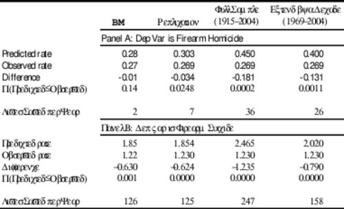
Note: Figures in the column headed ‘BM’ are taken directly from the text in Baker and McPhedran (2006). Replication shows our best attempts to produce the same results, using the same time period (1979-1996). Predicted rate is based on estimating an ARIMA model using data up to 1996, and forecasting out to 2004. Observed rate is the average in the data from 1996 to 2004. Lives saved per year is calculated by multiplying the difference (change in the rate per 100,000 people) by 200 (since the population of Australia is 20 million). The model estimates and predictions are from R.
Several points are notable. First, as expected, predicted firearm suicides and homicides after 1997 are considerably smaller when data from 1979 onwards is used, than when the full data set is used. The models estimated from the longer time series suggest that there were on average 250 fewer firearm deaths per year after the implementation of the NFA than would have been expected based on the predictions from the ARIMA model – close to double the numbers implied by Baker and McPhedran’s estimates.
A second key concern with the time period selected by Baker and McPhedran is that estimating an ARIMA(1,1,1) model using data only from 1979-1996 is dubious, especially for firearm homicides. The point estimates over the shorter time period are sensitive to the specification, and even to the statistical package used. This partly reflects the well-known difficulties associated with estimating an ARIMA model with such a short time series. However, it also reflects the fact that the ARIMA(1,1,1) model appears to be inappropriate in this case – simple statistical tests reject the hypothesis that Australian homicide rates follow a non-stationary process.[11] Baker and McPhedran present no statistical tests to show whether this model is appropriate. Augmented Dickey-Fuller tests, which are a simple way to determine whether a series is integrated (non-stationary), are shown in Appendix Table B2. They strongly reject the null hypothesis that the series are integrated in the case of firearm and non-firearm homicides.
Third, these results are not driven by some distant historical episode. The final column of Table 1 shows that even if we extend the sample period by only a decade, the probability that firearm deaths were not lower than would be expected based on a simple ARIMA(1,1,1) model is well below 1% for both homicides and suicides.
In modelling death rates, particularly where the absolute number of deaths is rather small, it is important to carefully consider whether the model used is appropriate to the task. Most empirical models of death rates consequently use an empirical specification appropriate to count data (Poisson or negative binomial) or take other steps to ensure that predicted death rates do not fall below zero (using the natural logarithm of the death rate as the dependent variable, or explicitly allowing for zero observations through a Tobit model, for instance).
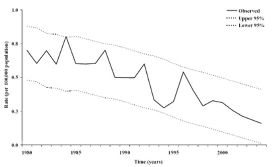
As the dependent variable, Baker and McPhedran (2006) use the number of deaths of a particular type per 100,000 people. If the firearm death rate were high and stable, this might not present a problem. However, since the firearm death rate is low and volatile, the estimates in Baker and McPhedran place a non-zero probability on the death rate for accidental firearm deaths and firearm homicides falling below zero. As is shown graphically in Figure 1 (which merely repeats figures 4A and 5 from Baker and McPhedran 2006), it cannot be rejected at the 95% confidence level that there will be negative deaths after 1994 for accidental firearm deaths, and after 2004 for firearm homicides. Projecting out further, the models predict that by 2010, deaths attributable to assault with a firearm or an accidental firearm incident would be negative. This is concerning: an effective modelling strategy should place a zero probability on the occurrence of a logically impossible event. Furthermore, it points clearly to the issue raised earlier of the low power of the tests. If, in order for Baker and McPhedran to be satisfied that firearm homicides fell after 1997, there must be a negative number of firearm homicides, then the test clearly has no statistical power.
|
Figure 1: Death Rates Cannot Fall Below Zero
|
 |
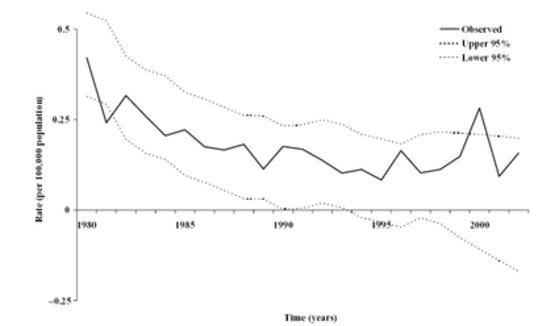 |
Note: Panels are from Baker and McPhedran (2006). First panel shows their Figure 4A (firearm homicide rate per 100,000 people) and the second panel shows their Figure 5 (accidental firearm death rate per 100,000 people).
There are straightforward and well-known solutions to this problem. In order to ensure that predicted death rates are always positive, researchers can use a Poisson model, or take the log of the rate, rather than the rate itself. Such approaches are common in studies of the impact of gun laws on deaths (see e.g. Ozanne-Smith et al 2004; Duggan 2001; Beautrais et al 2006; Chapman et al 2006). Indeed, we have been unable to find another study examining firearm-related deaths that simply uses the death rate as a dependent variable with no further specification checks.
We check the sensitivity of Baker and McPhedran’s results to the use of a log rather than a levels specification. Table 2 shows estimates of the post-1996 reduction in deaths, taken from ARIMA(1,1,1) models with the dependent variable as the log of the death rate, both for the period 1979-2004 and for the full period 1915-2004. The coefficient estimates are converted into level terms to facilitate comparison. The results show an increase in the predicted death rate in the log model compared with the levels models shown in Table 1. More importantly, though, there is a very clear reduction in the probability that the observed series is greater than the predicted series for firearm homicides in the model estimated from 1979 to 1996. The estimated probability that the predicted series is smaller than the actual series drops from 2.5% to 0.26% (compare the second columns of Table 1 and Table 2). Thus, there is extremely strong evidence in this model that the observed firearm homicide rate was lower after 1997 than would have been expected based on an ARIMA(1,1,1) log model estimated from 1979 to 1996.
Table 2: Comparison of predicted and observed rates of firearm homicide and suicide, ARIMA(1,1,1) model (dependent variable is the death rate)
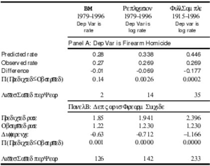
Note: Figures in the column headed ‘BM’ are taken directly from the text in Baker and McPhedran (2006). The other columns use the log of the death rate, rather than the death rate itself, as the dependent variable in the model estimated to obtain forecasts. These forecasts are then converted back to a death rate, to ensure comparability with Table 1. Model estimates and predictions are from R.
Note that a part of our concern with the model specification in Baker and McPhedran (2006) is the combination of the ARIMA(1,1,1) model – and in particular the assumption that the series are integrated –, the 1979 starting date, and the use of levels rather than logs. We present results from the ARIMA(1,1,1) models here, in order to show how sensitive the results are to even small specification changes. (The results from AR(1) models or from simple linear regression models that incorporate time trends typically yield point estimates of a similar or larger magnitude to those shown here.[12])
Here again, our criticism on model specification is unique to Baker and McPhedran’s analysis. Both Ozanne-Smith et al (2004) and Chapman et al (2006) use techniques (Poisson and negative binomial regression respectively) that rule out the possibility of negative deaths. In addition, the specification used by Chapman et al (2006) (allowing for both trend breaks and breaks in the level of the series) appears, if anything, to work against finding any effect of the NFA.
This article has reviewed the available evidence on the effects of Australia’s National Firearms Agreement on homicide and suicide rates. While we mainly focus on general methodological points, it is useful to consider whether we can confidently draw any conclusions from the three studies currently available.[13]
Although we can point to flaws in all three papers, we believe that Baker and McPhedran (2006) contains too many statistical and interpretive deficiencies, several of which are outlined above, to enable objective readers to rely on it to any extent. Chapman et al (2006) provide useful summary evidence on the trends in firearm and non-firearm deaths, and uniquely among the three, also some evidence on mass shooting events. Their empirical model is reasonable, although some testing of alternative specifications and time periods would have been helpful to the paper. If anything, their empirical strategy and use of 1979 as a starting point bias their results against finding a downward shift in firearm death rates coincident with the NFA. Ultimately, however, as the authors themselves acknowledge, they cannot be sure that any decline in firearm death rates after 1997 is causally related to the NFA.
Of the three, Ozanne-Smith et al (2004) have the most satisfying identification strategy, relying on an earlier policy change in Victoria and cross-state differences in firearm homicide and suicide rates to identify a plausibly causal effect of tighter firearm regulations. They find a 14% drop in death rates in the rest of Australia relative to Victoria after 1997, mostly due to lower firearm suicide. It is likely that this identification strategy too would have underestimated the effect of the NFA, since there is a reasonable possibility that the NFA had some effects in Victoria (a substantial number of guns were handed in by Victorians under the buy-back). A key weakness of the paper is that it does not consider whether there is evidence of method substitution. Further, recent advances in techniques for dealing with policy experiment studies with small numbers of policy changes (Bertrand et al 2004) suggest that there may be some concerns with the calculation of standard errors in that paper.
Given that the time series and other available evidence to date suggest a substantial fall in firearm deaths, can we say there was (likely) a decline in overall homicides and suicides following the NFA? Making such an inference would require a conclusion to be drawn on method substitution. Here, Ozanne-Smith et al (2004) provide no guidance; the best evidence we have to rely on is the time series evidence. In our view – and the views expressed in Baker and McPhedran (2006) and Chapman et al (2006) – the lack of any marked, sustained increase in non-firearm suicide or homicide rates after 1997 suggests there is little reason to suspect any long-run method substitution effect. It is, however, difficult to be certain of this without first having in place a model that satisfactorily explains movements in total deaths, and simple time-series models are not sufficient in this regard. Further, it would likely be difficult to identify method substitution if it occurred, given that in Australia, firearm deaths are small relative to total numbers of deaths and to the volatility in overall deaths. Despite these difficulties, and although we cannot rule out the possibility that non-firearm suicide and homicide would have fallen faster in the absence of the NFA, the fact that overall violent deaths have fallen since 1996 suggests there has not been substantial method substitution.
As we point out in our re-analysis of some of the findings in Baker and McPhedran (2006), the high degree of variability in the underlying data and the fragility of the estimated results with respect to different specifications and even statistical packages used, suggest that time series analysis alone cannot conclusively identify the effect of a national law change on death rates. However, to the extent that the available evidence points anywhere, it is towards the conclusion that the NFA reduced gun deaths.
The main thrust of this article, however, has been to raise some methodological concerns with the existing studies – in particular, regarding robustness to small changes in the time period and the model specification.
Aside from the question of the robustness of the results, a critical issue is whether time series analysis alone can ever be definitive in drawing conclusions about the effects of national policy changes. In the appendix to this article we show that it cannot, except under certain rather stringent assumptions. We do not believe that this means that such analysis is not worth undertaking or publishing. However, authors do need to be careful in interpreting their results.
Finally, it would be simple for researchers to make publicly available their statistical programs and data, allowing others to replicate their work. In two of the three papers we examine, researchers provide the full data set used in their empirical work in their paper, but even then it is difficult to replicate the results described in published papers because of uncertainties regarding the precise specification used.[14] The additional cost of making the data available in a package ready for statistical analysis and posting the statistical programs used to generate the final results (which in each case appears to have involved a single regression for each type of death examined) would be small. This would assist other researchers in satisfying themselves as to the validity of the results.[15]
We thank Jenny Mouzos for providing the data on firearm and non-firearm deaths used in the empirical analysis, and Don Weatherburn, Justin Wolfers, Azim Essaji, Paul Maxim, Susanne Schmidt and an anonymous referee for helpful comments on this article.
Baker J & McPhedran S 2006 ‘Gun Laws and Sudden Death: Did the Australian Firearms Legislation of 1996 Make a Difference?’ British Journal of Criminology Advance Access published on 18 October 2006 (doi:10.1093/bjc/azl084)
Beautrais AL, Ferguson DM & Horwood LJ 2006 ‘Firearms legislation and reductions in firearm-related suicide deaths in New Zealand’ Australian and New Zealand Journal of Psychiatry vol 40 pp 253-259
Bertrand M, Duflo E & Mullainathan S 2004 ‘How much should we trust difference-in-differences estimators?’ Quarterly Journal of Economics vol 119 no 1 pp 249-275
Britt CL, Kleck G & Bordua DJ 1996 ‘A reassessment of the DC gun law: some cautionary notes on the use of interrupted time series designs for policy impact assessment’ Law & Society Review vol 30 no 2 pp 361-380
Chapman S, Alpers P, Agho K & Jones M 2006 ‘Australia’s 1996 gun law reforms: faster fall in firearm deaths, firearm suicides and a decade without mass shootings’ Injury Prevention vol 12 no 6 pp 365-372
Duggan M 2001 ‘More Guns, More Crime’ Journal of Political Economy vol 109 no 5 pp 1086-1114
Kleck G 2001 ‘Impossible policy evaluation and impossible conclusions – a comment on Koper and Roth’ Journal of Quantitative Criminology vol 17 no 1 pp 75-80
Koper CS & Roth JA 2001a ‘The impact of the 1994 federal assault weapon ban on gun violence outcomes: an assessment of multiple outcome measures and some lessons for policy evaluation’ Journal of Quantitative Criminology vol 17 no 1 pp 33-74
Koper CS & Roth JA 2001b ‘A priori assertions versus empirical inquiry: a reply to Kleck’ Journal of Quantitative Criminology vol 17 no 1 pp 81-88
Kriesfeld R & Harrison J 2005 ‘Injury Deaths, Australia, 1999’ Injury Research and Statistics Series Number 24 (AIHW cat. no. INJCAT 67) AIHW Adelaide
McCloskey DN & Ziliak ST 1996 ‘The Standard Error of Regressions’ Journal of Economic Literature vol 34 no 1 pp 97-114
McDowall D & Loftin C 2005 ‘Are U.S. crime rate trends historically contingent?’ Journal of Research in Crime and Delinquency vol 42 no 4 pp 359-383
McDowall D 2002 ‘Tests of nonlinear dynamics in U.S. homicide time series, and their implications’ Criminology vol 40 no 3 pp 711-735
Ozanne-Smith J, Ashby K, Newstead S, Stathakis VZ & Clapperton A 2004 ‘Firearm related deaths: the impact of regulatory reform’ Injury Prevention vol 10 pp 280-286
Reuter P & Mouzos J 2003 ‘Australia: A Massive Buyback of Low-Risk Guns’ in Ludwig J & Cook PJ (eds) Evaluating Gun Policy: Effects on Crime and Violence (pp 121-156) Washington, DC
The following discussion is framed in terms of suicide, where method of choice has been more commonly studied, but the analysis could be applied equally to murder. It is described in terms of firearm and hanging, simply to make the model more concrete and relevant to the issues discussed in this paper. Suppose these are the only two possible forms of suicide, and that numbers of suicides per year in a particular country are determined by:
Firearmt = α1 + β1Xt + ρ1gunst + εt (1)
Hangingt = α2 + β2Xt + ρ2gunst + υt (2)
We assume that there are sufficient numbers of deaths that the errors are approximately normally distributed, and that there is no serial correlation in the error terms. We also assume that cov(εtυt) = 0.
In this simple model, there are thus two reasons why firearm and hanging deaths may be related to each other. First, movements in Xt cause changes in deaths. This variable is intended as a simple representation of what Baker and McPhedran (2006) refer to as the ‘political, social and economic culture’, which may affect the decision to suicide. Suppose, for instance, that increases in the unemployment rate increase the numbers of suicides – then Xt is the unemployment rate and β1 and β2 would be positive. For the purposes of evaluating the effect of changes in the gun laws, we are not concerned about these coefficients, except that we want to ensure that we do not mis-attribute falls in firearm-related suicides to general social changes.
The variable gunst represents the legal environment around gun ownership. The model above allows that changes in gun laws may have led to changes in both firearm and hanging suicides. The simple intuition that drives tightening of gun laws is typically that ρ1 would be negative: a tightening of gun laws would reduce firearm-related suicides. However, there is a possibility that method substitution may occur, so that changes in gun laws that reduce firearm-related suicides may actually increase suicides by hanging.
Given this model, total suicides are:
Suicidet = Firearmt + Hangingt
= (α1+α2)+ (β1+β2)Xt + (ρ1+ ρ2)gunst + (εt + υt)
= (α1+α2)+ (β1+β2)Xt + (ρ1+ ρ2)gunst + μt (3)
The central questions for this paper are:
(1) is ρ1 negative? (did firearm-related deaths fall after the change in laws?);
(2) is ρ2 positive? (was there method substitution?); and
(3) is (ρ1 + ρ2) negative? (did overall suicides fall after the change in laws?)
A way of determining this would be to estimate a stacked model:
Firearmt
= α1 + β1Xt + ρ1gunst + α2Ht + β2(Ht Xt)+ ρ2(Htgunst)+ μt (3)
Hangingt
Suppose, however, that we have no information on X available to us. Can we answer these questions? There are two possibilities. First, if β1 = β2, then there is a potentially simple solution: subtract hangings from firearm deaths, so that we have:
Firearmt – Hangingt = (α1 – α2) + (β1 – β2) Xt + (ρ1 – ρ2)gunst + (εt + υt)
= (α1 – α2) + (ρ1 – ρ2)gunst + (εt + υt) (4)
In this case, however, we will only be able to test the third of the propositions – we will not be able to say anything about the impact on firearm-related suicides, or on method substitution – and that only implicitly by assuming that ρ1 <0 and that ρ2 >=0. The assumption that firearm and hanging deaths respond in the same way to the same stimuli is also unsatisfactory.[16] For example, if unemployment rates affect suicides in low-income families more than in high-income families, but firearms tend to be owned by high-income families, then β1 ≠ β2.
What if we simply omit Xt and perform the stacked regression analysis described in (3)? Then we have:
Firearmt
= α1 + ρ1gunst + α2Ht + ρ2(Htgunst)+ ζt (5)
Hangingt
where ζt = β1Xt + β2(Ht Xt)+ μt. Estimates of ρ1 and ρ2 will be biased and inconsistent if there is any correlation between Xt and gunst. Given the particular nature of this model, where there is only time series variation, and where gunst is a dummy equal to one after 1997, this is inevitable if there is any time-series variation in Xt. This is roughly similar to the problem of using a difference-in-difference estimator with time series variation and serial correlation as described in Bertrand et al (2004), except that in this case the lack of a reasonable control group exacerbates the difficulties. Suppose, for instance, that a drought tends to lead to higher firearm suicides, but not higher suicides by hanging (Xt is drought, β1 > 0, β2 = 0). Then the Australian drought of the mid-2000s should have led to more firearm suicides, but not hangings. Failing to account for this in estimating (5) would see all those excess suicides attributed to the NFA; that is, the estimate of ρ1 would be biased in a positive direction.
In short, time series variation in and of itself is unable to recover plausible estimates of the effect of the Australian gun laws on deaths, except in the presence of extremely restrictive (and probably inaccurate) assumptions on the determinants of the numbers of deaths. Without having some credible control group – or at a minimum a model that introduces time-varying factors that affect homicide and suicide rates, such as personal income growth, unemployment rates, or health and social program changes – we can draw no definitive conclusions on either the extent of method substitution, or on the underlying direction of overall homicide and suicide rates.
Appendix B. Details of Regression Results
A (1,1,1) models of firearm and non-firearm suicides and homicides
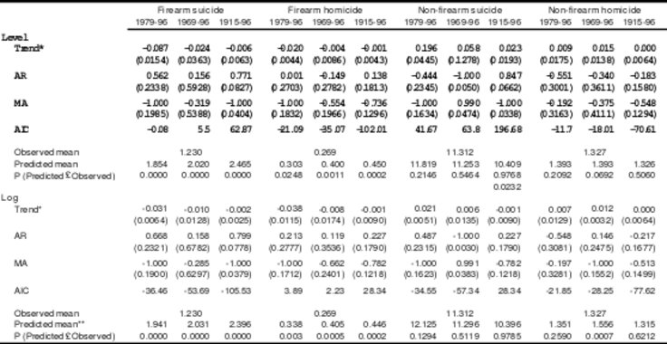 Table B1:
Estimates from ARIM
Table B1:
Estimates from ARIM
* The estimated trend is the constant in the first-differenced model.
** For ease of interpretation, predictions for the log models were converted to levels for calculating the means and conducting the t-tests.
Coefficients in bold are significant at the 5% level.
Table B2: Augmented Dickey Fuller test results
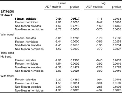
Note: Coefficients in bold are significant at the 5% level. This indicates that there is substantial evidence against the null hypothesis that the series is integrated. That is, it indicates that an I(1) model is inappropriate for the particular series. Typically, the preferred ADF test statistic is one based on a model that allows for a time trend.
[∗] Corresponding author. Department of Economics, Wilfrid Laurier University, 75 University Ave West, Waterloo, ON, N2L 3C5, Canada. Email cneill@wlu.ca. Website: www.wlu.ca/sbe/cneill
[**] Research School of Social Sciences, Australian National University, Canberra, Australia. Email: andrew.leigh@anu.edu.au. Website: andrew.leigh@anu.edu.au
[1] Data going back to 1979 at the national level are available from Australian Bureau of Statistics (ABS) publications, but earlier data must be purchased from ABS Consultancy Services.
[2] Chapman et al (2006) exclude data after 2003 from their analysis, based on concerns over data reliability. The number of deaths identified in each year differs somewhat between Chapman et al (2006) and Baker and McPhedran (2006). It is unclear why this is the case.
[3] ARIMA(1,1,1) refers to an auto-regressive integrated moving-average model, with integration of order 1 and first-order serial correlation and moving average components.
[4] Chapman et al do not estimate the statistical significance of this difference, but given the prior history of mass shootings in Australia, the probability that this change in the frequency of mass shootings was due to mere chance is well below 1%.
[5] In the case of the gun buy-back, this assumption is clearly violated. Reuter and Mouzos (2003:132) show that the number of firearms handed back in Victoria in 1997 was 4,300 per 100,000 people, a higher rate than for Australia as a whole (3,400 per 100,000 people).
[6] This is broadly the conclusion in their published paper. Statements to the media, however, were much stronger. In a summary of the research released at the Sporting Shooters’ Association of Australia website, the conclusions are:
• ‘The reforms did not affect rates of firearm homicide in Australia.
• The reforms could not be shown to alter rates of firearm suicide, because rates of suicide using other methods also began to decline in the late 1990s.
• …
• It must be concluded that the gun buyback and restrictive legislative changes had no influence on firearm homicide in Australia.
• The lack of effect of a massive buyback and associated legislative changes in the requirements for obtaining a firearm licence or legally possessing a firearm has significant implications for public and justice policy, not only for Australia, but internationally.’
Source: ‘Gun Laws and Sudden Death: Did the Australian Firearms Legislation of 1996 Make a Difference? Executive Summary’. Available online on 18 December 2007, from www.ic-wish.org/Executive%20Summary.pdf
[7] Koper and Roth are clearly aware of these difficulties, and highlight them in their paper, noting that ‘the law has not produced a clear impact on gun violence’ (2001a:69), although they suggest that the ban likely ‘contributed to a reduction in gun homicides’ (2001a:33).
[8] Although much of Kleck (2001) focuses on the relatively small impact that the 1994 US federal ban on assault weapons and large capacity magazines had on overall gun ownership (a critique that is not applicable to the Australian NFA), Kleck concludes by saying ‘there is no effective way to assess the impact on crime rates of a unique national policy change’ (2001: 80). This critique is potentially applicable to the Australian reform.
[9] An exception is Chapman et al (2006), who exclude data from 2004 that was considered to be of dubious quality. No results are reported in that paper from different time periods, however.
[10] We could not obtain the full set of data underlying Figures 1 and 2 in Baker and McPhedran (2006) from the corresponding author. Our results are therefore based upon Table 1 in Baker and McPhedran (2006), supplemented with data kindly provided by Jenny Mouzos of the Australian Institute of Criminology, and the most recent population data from the Australian Bureau of Statistics. We first used precisely the data laid out in Baker and McPhedran (2006) and estimated ARIMA(1,1,1) models for the period 1979 to 1996. We did not have access to the same statistical package used by Baker and McPhedran, and initially used STATA. STATA did not yield estimates similar to those reported by Baker and McPhedran. For instance, the firearm homicide model did not converge. Simply changing the population figures to more recent ABS estimates helped somewhat. Switching to the statistical package R brought our estimates considerably closer to those in Baker and McPhedran; the results reported here are therefore from R. We consider the estimates from R to be more reliable, but the sensitivity of the estimates to the statistical package used is somewhat concerning, and itself suggests that the ARIMA(1,1,1) specification is not ideal. Note, however, that regardless of the statistical package used, and despite coming quite close on firearm suicides, we could not replicate Baker and McPhedran’s predictions of the average firearm homicide rate after 1997 in the absence of the NFA. We also note that the statistical ‘test’ used by Baker and McPhedran is more heuristic than formal. McDowall and Loftin (2005) discuss more formal tests for structural breaks in an I(1) model. Here, we nonetheless use the methods described in Baker and McPhedran, in order to focus attention on the robustness of the results to modelling changes. All data used in this paper and the programs used to obtain the statistical results (in STATA and R), as well as details of those results in numerical and graphical form, are available at www.wlu.ca/sbe/cneill.
[11] McDowall (2002) notes that to date little attention has been paid to the possibility that crime rates can be described by non-stationary processes. Using a time series from 1925 to 2000, described in McDowall and Loftin (2005) as ‘short’, he finds that US homicide rates are well-described by an I(1) model with first-order serial correlation.
[12] Results available on request.
[13] In principle, a variety of statistical approaches could be used to model the effect of the NFA on firearm deaths. Exploring the full gamut of approaches may be a useful exercise, but it is beyond the scope of this paper.
[14] The term ‘replicate’ has been the subject of some recent controversy. Here, we use it in its most limited sense, to mean recovering the same estimates in a published paper using the same data set. We see such ‘replication’ as a first, rather than a final, step in assessing a paper’s conclusions.
[15] All data and statistical programs used in this paper are available at: www.wlu.ca/sbe/~cneill
[16] This is the concern that Britt et al (1996) have with the use of non-firearm deaths as a control for firearm deaths.
AustLII:
Copyright Policy
|
Disclaimers
|
Privacy Policy
|
Feedback
URL: http://www.austlii.edu.au/au/journals/CICrimJust/2008/22.html